The Curse of Dimensionality
AI InsightsMany machine learning practitioners may have come to a crossroads where they have to choose the number of features they want to include in their model. This decision is actually dependent on many factors. For instance, you may need to know about the nature of your data, is the feature contributing (is it some kind of ID)? Are features multi-collinear? How many samples do you have? Machine Learning practitioners often work with high dimensional vectors to create a model. Since dimensions higher than k=3 are impossible to visualize, it is often hard for us to know if our model construct is right or wrong. In this post, I will illustrate the Curse of Dimensionality, a powerful concept where the volume of the vector space grows exponentially with the dimension, causing our data to be highly sparse and distant from one another, and discuss its implications to the work of data science.
High Dimensional Spaces
Let’s illustrate the vastness of a high dimensional space by considering a hypersphere inside a hypercube. In two or three dimensions, they look like this
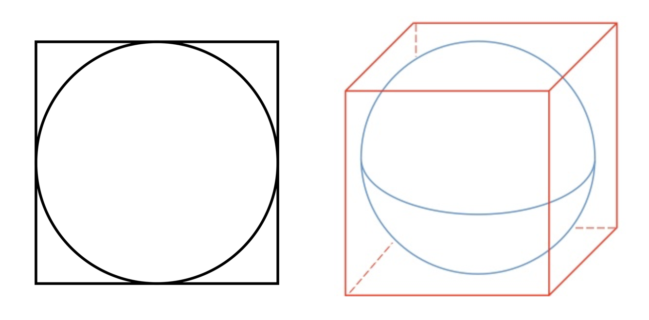
Although not visualizable in higher dimensions, we can generalize the concept of a hypersphere inside a hypercube in any N dimensions.
Now let’s consider a hypercube of side s=2r where r is the radius of the hypersphere. To show how fast the space grows, I will consider the volume of hypercube to hypersphere ratio. If the hypersphere eats up more volume as the dimension grows, then the ratio should converge to 1. Conversely, if the hypersphere eats up less volume as the dimension grows, then the ratio should converge to 0. (Spoiler: As explained here, the analytic solution is the ratio should converge to 0.)
Monte Carlo Simulation
Here, we will do a Monte Carlo simulation to show that this is true. First we sample a data point from a uniform random distribution in k dimensions. Then we calculate the Euclidean Distance of this point from the origin; if the distance is lower than r, then the point lies inside the hypersphere with radius r, and vice versa. We calculate the fraction of the times this occurs. You can find the code of this experiment in my github. The result is shown as follows:
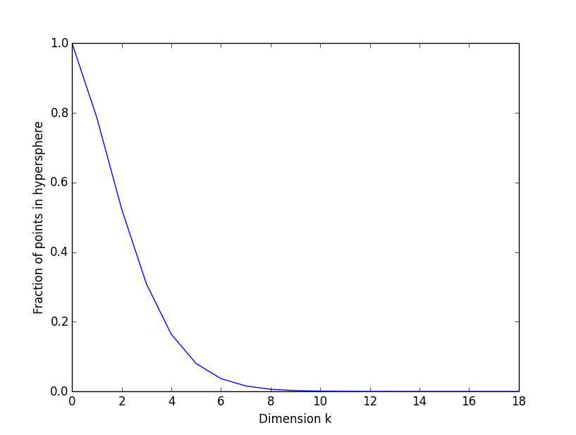
In the plot above, the x-axis is the number of dimensions, and the y-axis is the volume of hypersphere to volume of hypercube ratio. A simple run with 1 million samples from a k-dimensional uniform random distribution, where k ranges from 1 to 100, gives the following statistics.
k = 1
Volume of hypercube = 2
Fraction of points inside hypersphere = 1.0
-----------------------------------------
k = 2
Volume of hypercube = 4
Fraction of points inside hypersphere = 0.784976
-----------------------------------------
k = 3
Volume of hypercube = 8
Fraction of points inside hypersphere = 0.52376
-----------------------------------------
...
k = 17
Volume of hypercube = 131072
Fraction of points inside hypersphere = 1e-06
-----------------------------------------
k = 18
Volume of hypercube = 262144
Fraction of points inside hypersphere = 0.0
-----------------------------------------
k = 19
Volume of hypercube = 524288
Fraction of points inside hypersphere = 0.0
-----------------------------------------
Discussion
In the experiment above, notice that we start with a 1. This intuitively makes sense because in one dimension all we have is a line of length 1, so the hypersphere is the same as the line. From there, the fraction decreases exponentially, and converges to 0. This has a powerful implication to data scientists that if you increased your data’s dimensionality, you’d need exponentially more data to compensate for the vastness of the space (i.e. sparseness of the data), and this may lead to overfitting. Therefore, next time when you consider adding more features to your data/model, do consider the potential problems that might arise when your dimension becomes too big. Finally, I encourage you to play around with the code and change some parameters to see this effect for yourself!
Contact us
Drop us a line and we will get back to you

